Mining the screenplay of The Room

25 Jan 2018

While sitting in the office, my colleague Brian and I stumbled upon this dead-on honest trailer of The Room a.k.a. one of the worst movies of all time (written, produced, directed by and starring Tommy Wiseau).

And since the movie features such Shakespearian quotes as “I did not hit her, it’s not true! It’s bullshit! I did not hit her! I did naaht! Oh hi, Mark”, we joked about mining the screenplay for other hidden gems.

Well, no sooner said than done.

Setup

Conducting the analysis below requires the packages dplyr, ggplot2, magrittr, pdftools, reshape2, stringr, tidytext, and wordcloud.

For loading multiple packages at once I recommend p_load() from the pacman package which is a wrapper function for library() and require() and installs missing packages if necessary.

# Install and load pacman if not already installed
if (!require("pacman")) install.packages("pacman")
library(pacman)

# Load packages
p_load(dplyr, ggplot2, magrittr, pdftools, reshape2, stringr, tidytext, wordcloud)

Importing data

The full movie script can be found here. To download and import it to R, simply run

# Download pdf
download.file("https://theroomscriptblog.files.wordpress.com/2016/04/the-room-original-script-by-tommy-wiseau.pdf",
              "the-room-original-script-by-tommy-wiseau.pdf")
              
# Extract text from pdf file
room <- pdf_text("the-room-original-script-by-tommy-wiseau.pdf")

and extract the text via pdf_text() from the package pdftools.

Text cleaning

After extracting the raw text from The Room’s pdf screenplay it needs some cleaning prior to analyzing.

Concretely, this means separating the lines of the raw text (\n indicating line breaks), removing redundant text parts such as the cover page, headers and footers, blank lines, and directing instructions as well as punctuation (except for apostrophes), non-alphabetic characters, and stopwords. (Note that I deliberately didn’t stem words.)

For most of these steps lapply() can be used to apply the respective functions to each element of the list.

While performing these steps, the cleaned text, which consists of a sequence of strings, is split into single words – a process called tokenization.

# Separate lines with \n indicating line breaks
room_tidy <- strsplit(room, "\n")

# Remove cover page
room_tidy <- room_tidy[-1]

# Remove page numbers and headers
room_tidy <- lapply(room_tidy, function(x) x[-(1:2)])

# Remove footers
room_tidy <- lapply(room_tidy, function(x) x[1:(length(x)-2)])

# Remove information on act and scene
room_tidy <- lapply(room_tidy, function(x) gsub("END SCENE", "", x))
room_tidy <- lapply(room_tidy, function(x) gsub("ACT.*", "", x))
room_tidy <- lapply(room_tidy, function(x) gsub("SCENE.*", "", x))

# Remove punctuation (except for apostrophes) and numbers
room_tidy <- lapply(room_tidy, function(x) gsub("[^[:alpha:][:blank:]']", "", x))

# Remove directing instructions
room_tidy <- lapply(room_tidy, function(x) x[!grepl("^[A-Z ']+$", x), drop = FALSE])

# Convert to lowercase
room_tidy <- lapply(room_tidy, function(x) tolower(x))

# Split strings
room_tidy <- lapply(room_tidy, function(x) strsplit(x, " "))

# Turn list to data.frame 
room_df <- data.frame(matrix(unlist(room_tidy), nrow = 10357, byrow = T), stringsAsFactors = FALSE)

# Remove introductory part and last two lines
room_df <- tail(room_df, -102)
room_df <- head(room_df, -2)

# Rename column to match anti_join(stopwords)
colnames(room_df) <- "word"

# Remove blank lines from text
room_df %<>% filter(word != "") 

# Remove stopwords
room_df %<>% anti_join(stop_words)

Visualizing word frequencies

After processing the raw text and turning it into a tidy format we can extract the most common words from the movie script by counting their appearances via count() from the plyr package and plot them by running the following code

# Find most common words
room_df_wordfreq <- room_df %>%
  count(word, sort = TRUE)

# Plot words
room_df %>%
  count(word, sort = TRUE) %>%
  filter(n > 20) %>%
  mutate(word = reorder(word, n)) %>%
  ggplot(aes(word, n)) +
  geom_col() +
  xlab("") + ylab("") + ggtitle("Most common words in The Room", subtitle = "Written by Tommy Wiseau") +
  ylim(0, 100) + coord_flip()

which creates this graph:

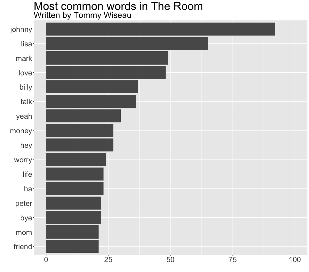
It comes as little surprise that the most common words in the movie script are of a similar quality to the quote in the beginning of this post with the most frequently used words being “Johnny”, “Lisa”, and “Mark” – the main characters’ names – and more elaborate expressions such as “yeah” or “ha” (sadly, naaht didn’t make it to the list).

Sentiment analysis

In a similar manner, we can conduct a basic sentiment analysis and visualize the results. For this purpose we will use the get_sentiments() function from the tidytext package and use both the NRC Emotion Lexicon from Saif Mohammad and Peter Turney (all sentiments) and the sentiment lexicon from Bing Liu and collaborators (positive/negative sentiments).

# Plot total sentiment scores (nrc)
room_df %>%
  inner_join(get_sentiments("nrc")) %>%
  count(word, sentiment) %>%
  ggplot(aes(sentiment, n)) +
  geom_bar(aes(fill = sentiment), stat = "identity") +
  theme(text = element_text(size = 30), axis.text.x = element_text(angle = 65, vjust = 0.5)) +
  xlab("") + ylab("") + ggtitle("Total sentiment scores in The Room", subtitle = "Written by Tommy Wiseau") +
  ylim(0, 500) + theme(legend.position = "none") 

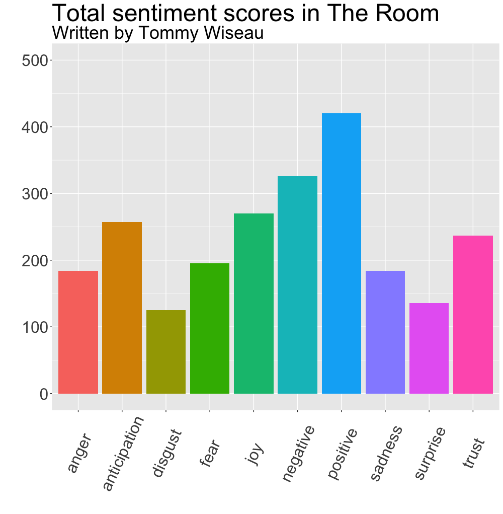
We can see in the NRC sentiments plot that most words in The Room’s screenplay are positively scored, followed by negatively scored words.

Positive and negative words

By calculating Bing sentiment scores next, we can explore the previous finding further.

# Calculate contributions to positive and negative sentiments (bing) by word 
bing_counts <- room_df %>%
  inner_join(get_sentiments("bing")) %>%
  count(word, sentiment, sort = TRUE) %>%
  ungroup()

# Calculate top word contributors
bing_counts_plot <- bing_counts %>%
  group_by(sentiment) %>%
  top_n(10) %>%
  ungroup() %>%
  mutate(word = reorder(word, n)) 

# Plot most common positive and negative words
ggplot(bing_counts_plot, aes(word, n, fill = sentiment)) +
  geom_col(show.legend = FALSE) +
  facet_wrap(~sentiment, scales = "free_y") +
  xlab("") + ylab("") + 
  ggtitle("Most common positive and negative words in The Room", subtitle = "Written by Tommy Wiseau") +
  coord_flip()

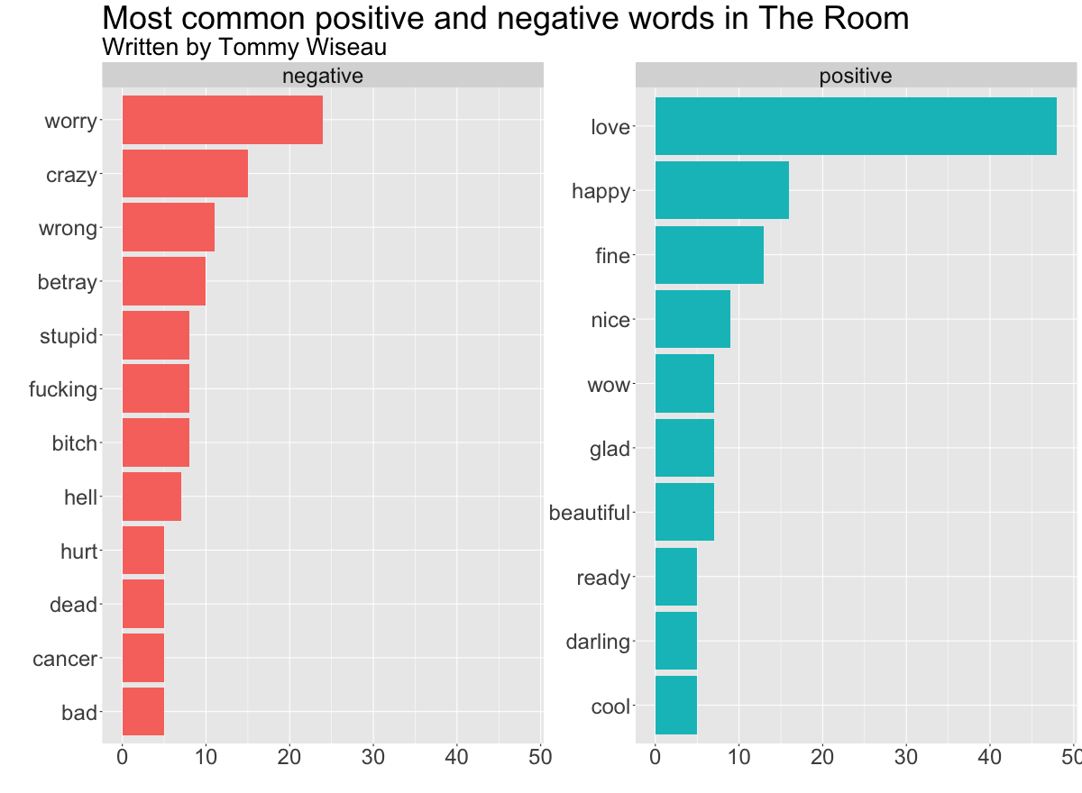
As the second sentiment graph shows, the most common positive words in The Room are “love”, “happy”, and “fine”, while the most common negative words are “worry”, “crazy”, and “wrong”.

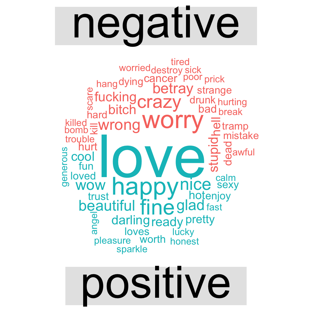
Word clouds

To finish it up, we now finally plot one of the infamous word clouds (albeit in a slightly more advanced version) by contrasting the most common positive words with the most common negative ones,

# Plot comparison cloud in ggplot2 colors
## Run > unique(g$data[[1]]["fill"]) after ggplot_build() to extract colors
room_df %>%
  inner_join(get_sentiments("bing")) %>%
  count(word, sentiment, sort = TRUE) %>%
  acast(word ~ sentiment, value.var = "n", fill = 0) %>%
  comparison.cloud(colors = c("#F8766D", "#00BFC4"), max.words = 60)

yielding this beautifully crafted word cloud:

Wrapping it up, the findings of this analysis can be summarized as follows:

Lisa Hehnke