Lisa Hehnke
Into the Unknown: Mining and visualizing STARSET song lyrics
03 Feb 2018
While browsing the datanet earlier this week, inspiration hit me when I stumbled across John MacKintosh’s awesome text analysis of Metallica lyrics using the equally awesome geniusR package by Josiah Parry.
In an instant, I decided to do my own song lyrics analysis featuring one of my favourite bands: STARSET, an American cinematic rock band formed by scientist turned lead singer Dustin Bates in 2013.
Since the band’s concept revolves around space, I thought it was a good fit to incorporate an element inspired by Nicholas Rougeux’s literary constellations into the analysis by creating starplot graphs, depicting pairs of adjacent words on an image of the Milky Way:
Enough said, here comes the code.
Setup
Reproducing this analysis requires the packages listed below. You can install and load them at once with p_load(), a wrapper function for library() and require() from the pacman package.
In addition, you have to install geniusR from GitHub with devtools.
# Install geniusR
install.packages("devtools")
library(devtools)
devtools::install_github("josiahparry/geniusR")
library(geniusR)

# Install and load the other packages with pacman
if (!require("pacman")) install.packages("pacman")
library(pacman)

# Load packages
p_load(ggraph, ggrepel, ggthemes, grid, igraph, jpeg, magrittr, reshape2, tidyr, tidytext, tidyverse, wordcloud)
Downloading song lyrics
geniusR provides an easy way to access lyrics as text data using the website Genius. To download the song lyrics for each track of a specified album you can use the genius_album() function which returns a tibble with track number, title, and lyrics in a tidy format.
I did this for both STARSET’s debut album Transmissions and its successor, Vessels.
# Download Transmissions album lyrics
transmissions <- genius_album(artist = "Starset", album = "Transmissions", nested = FALSE)

# Download Vessels album lyrics
vessels <- genius_album(artist = "Starset", album = "Vessels", nested = FALSE)

# Add columns for album and merge
transmissions$album <- "Transmissions"
vessels$album <- "Vessels"
starset <- rbind(transmissions, vessels)
Cleaning the text and setting the theme
Some minor data cleaning needed to be done first before starting with the actual analysis. Note, however, that I didn’t stem the words as stemming in this case occasionally messed up the words’ meanings so I left it out when revising the final code.
Additionally, I set up a customized ggplot2 theme and a color palette consisting of most colors from the Vessels album cover for the graphs.
# Remove punctuation (except for apostrophes) and numbers
starset$text <- gsub("[^[:alpha:][:blank:]']", "", starset$text)

# Unnest and tokenize text
starset_tidy <- starset %>%
  unnest_tokens(word, text) %>%
  anti_join(stop_words)

# Set theme for visualizations
viz_theme <- theme(
  strip.background = element_rect(colour = "grey20", fill = "#92a1a9"),
  axis.line = element_line(colour = "grey20"),
  panel.grid.major = element_blank(),
  panel.grid.minor = element_blank(),
  panel.border = element_blank(),
  panel.background = element_blank(),
  strip.text = element_text(size = rel(1), face = "bold"),
  plot.caption = element_text(colour = "#4e5975"),
  text = element_text(family = "Avenir"))

# Color palette based on Vessels album cover
starset_cols <- c("#363241", "#3b2d2d", "#483845", "#4d3b4b", "#332f3e", "#2a2a2c", "#353140", "#2c2a37", "#2f282f", "#363346", "#806c88", "#2f3b4b", "#282832", "#293241", "#245d68", "#1c2f36", "#16211d", "#172a31", "#0b2735", "#0d2434", "#102d3d", "#295860", "#1f383d", "#232f25", "#162f34", "#0b1e2f", "#192e43", "#133654", "#12202b", "#253b48", "#101a1b", "#223941", "#0e1b24", "#101922", "#0d1a23", "#0e1619", "#131418", "#10171d")
Visualizing word frequencies
The first step of the song text analysis consisted of calculating word frequencies and extracting the most common words on both albums.
# Plot most common words
starset_tidy %>%
  group_by(album) %>%
  count(word, sort = TRUE) %>%
  filter(n > 10) %>%
  top_n(10, n) %>%
  ungroup() %>%
  mutate(word = reorder(word, n)) %>%
  ggplot(aes(word, n)) +
  geom_segment(aes(x = word,
                   xend = word,
                   y = 0,
                   yend = n), col = "grey50", alpha = 0.9) +
  geom_point(col = starset_cols[1:17], size = 4, alpha = 0.9) +
  facet_wrap( ~ album, scales = "free_y", ncol = 2) +
  theme(text = element_text(size = 20, color = "#1f232e")) +
  xlab("") + ylab("") + ggtitle("Most common words on STARSET albums", subtitle = " ") +
  ylim(0, 60) + coord_flip() + viz_theme

ggsave("plot1.png", width = 12, height = 8, units = "in", dpi = 100)
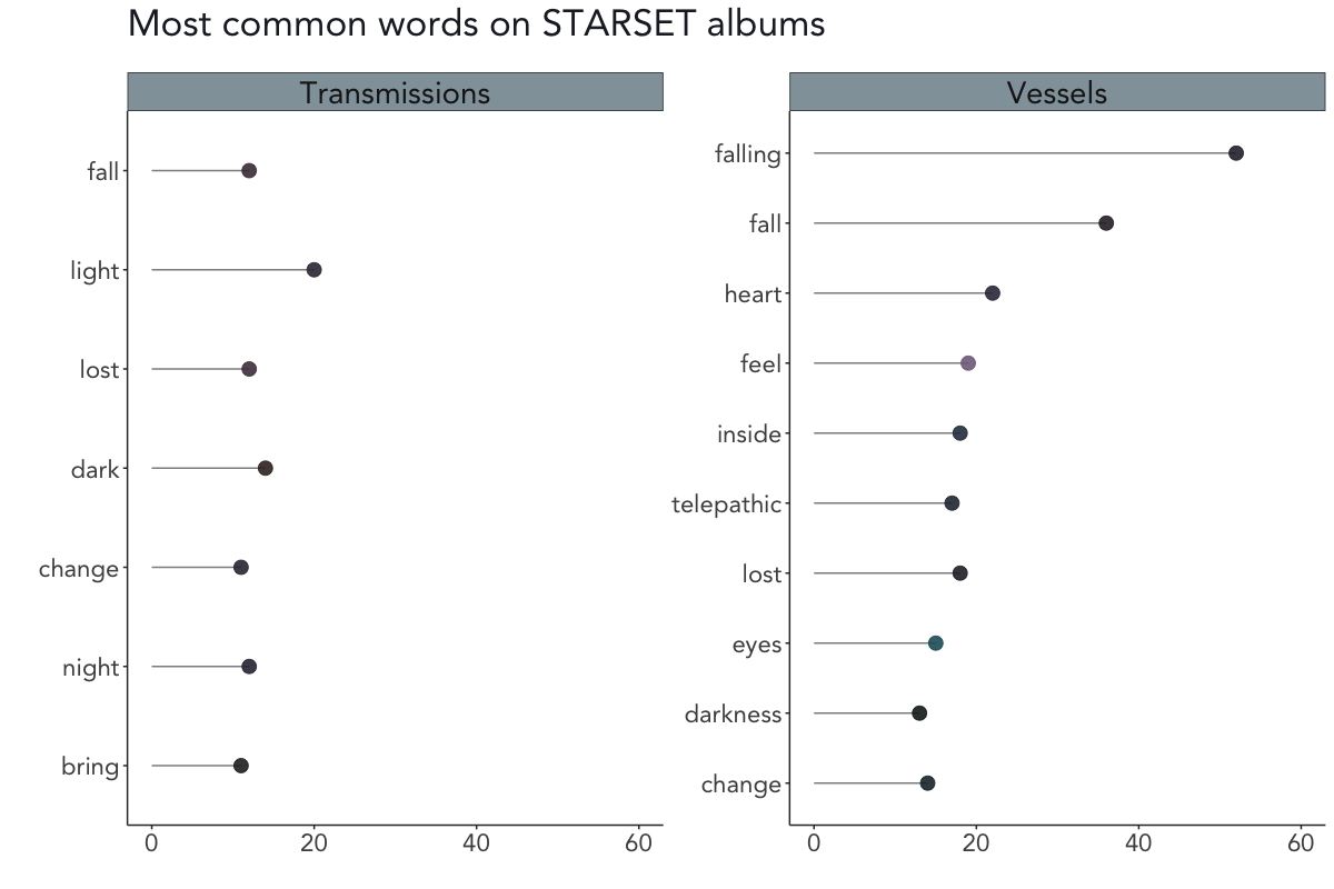
As you can see in the above plot, light (20x), dark (14x), and the trio fall/lost/night (each occurring 12 times) are the most common words on Transmissions, whereas falling (52x), fall (36x), and heart (22x) are the most common words on Vessels.
Sentiment analyses
For the next step of the analysis, I followed the proceedings from when I mined the screenplay of The Room in a previous post and evaluated the emotions in STARSET’s song lyrics using the NRC sentiment lexicon. NRC categorizes words into positive and negative categories as well as in anger, anticipation, disgust, fear, joy, sadness, surprise, and trust.
Getting sentiments using the NRC lexicon
# Plot NRC sentiment scores
starset_tidy %>%
  group_by(album) %>%
  inner_join(get_sentiments("nrc")) %>%
  count(word, sentiment) %>%
  ggplot(aes(sentiment, n)) +
  geom_bar(aes(fill = sentiment), stat = "identity", alpha = 0.9) +
  scale_fill_manual(values = starset_cols[25:35]) +
  facet_wrap( ~ album, scales = "free_y", ncol = 2) +
  theme(text = element_text(size = 20, color = "#1f232e"), axis.text.x = element_text(angle = 65, vjust = 0.5)) +
  xlab("") + ylab("") + ggtitle("Sentiment scores for STARSET albums", subtitle = " ") +
  ylim(0, 300) + theme(legend.position = "none") + viz_theme

ggsave("plot2.png", width = 12, height = 8, units = "in", dpi = 100)
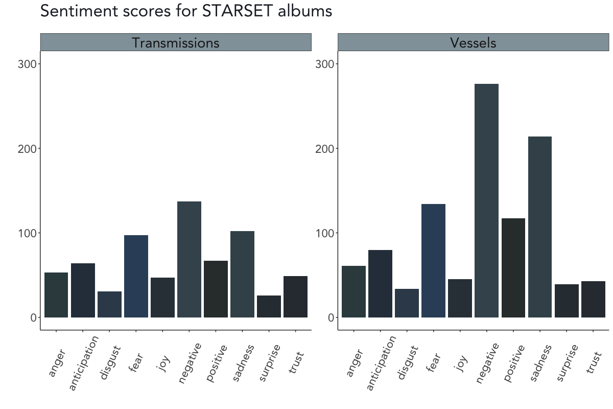
According to the NRC sentiment analysis, the emotions on both Transmissions and Vessels are – somewhat unsurprisingly for a rock band – rather negative, accompanied by mainly sadness and fear (although there’s a stronger hint of positivity on Vessels).
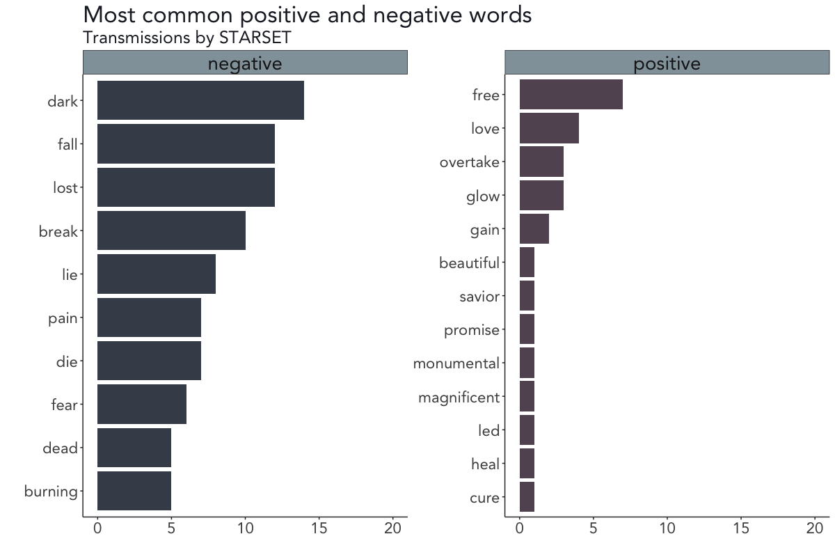
Getting sentiments using the Bing lexicon
After obtaining the results of the NRC sentiment analysis, I decided to dig deeper into STARSET’s alleged negativity (disclaimer: they’re obviously still a great band) by conducting another brief sentiment analysis using the Bing lexicon to extract the most common positive and negative words on both albums.
# Calculate Bing sentiment scores
starset_bing <- starset_tidy %>%
  group_by(album) %>%
  inner_join(get_sentiments("bing")) %>%
  count(word, sentiment, sort = TRUE) %>%
  ungroup()

# Get top word contributors
starset_bing_top <- starset_bing %>%
  group_by(album, sentiment) %>%
  top_n(10) %>%
  ungroup() %>%
  mutate(word = reorder(word, n))

# Plot most common positive and negative words: Transmissions
starset_bing_top %>%
  filter(album == "Transmissions")  %>%
  mutate(word = reorder(word, n)) %>%
  ggplot(aes(word, n, fill = sentiment)) +
    geom_col(alpha = 0.9, show.legend = FALSE) +
    facet_wrap(~sentiment, scales = "free_y") +
    scale_fill_manual(values = starset_cols[c(14, 4)]) +
    xlab("") + ylab("") +
    theme(text = element_text(size = 20, color = "#1f232e")) +
    ggtitle("Most common positive and negative words", subtitle = "Transmissions by STARSET") +
    ylim(0, 20) + coord_flip() + viz_theme

ggsave("plot3.png", width = 12, height = 8, units = "in", dpi = 100)

# Plot most common positive and negative words: Vessels
starset_bing_top %>%
  filter(album == "Vessels")  %>%
  mutate(word = reorder(word, n)) %>%
  ggplot(aes(word, n, fill = sentiment)) +
    geom_col(alpha = 0.9, show.legend = FALSE) +
    facet_wrap(~sentiment, scales = "free_y") +
    scale_fill_manual(values = starset_cols[c(14, 4)]) +
    xlab("") + ylab("") +
    theme(text = element_text(size = 20, color = "#1f232e")) +
    ggtitle("Most common positive and negative words", subtitle = "Vessels by STARSET") +
    ylim(0, 60) + coord_flip() + viz_theme

ggsave("plot4.png", width = 12, height = 8, units = "in", dpi = 100)
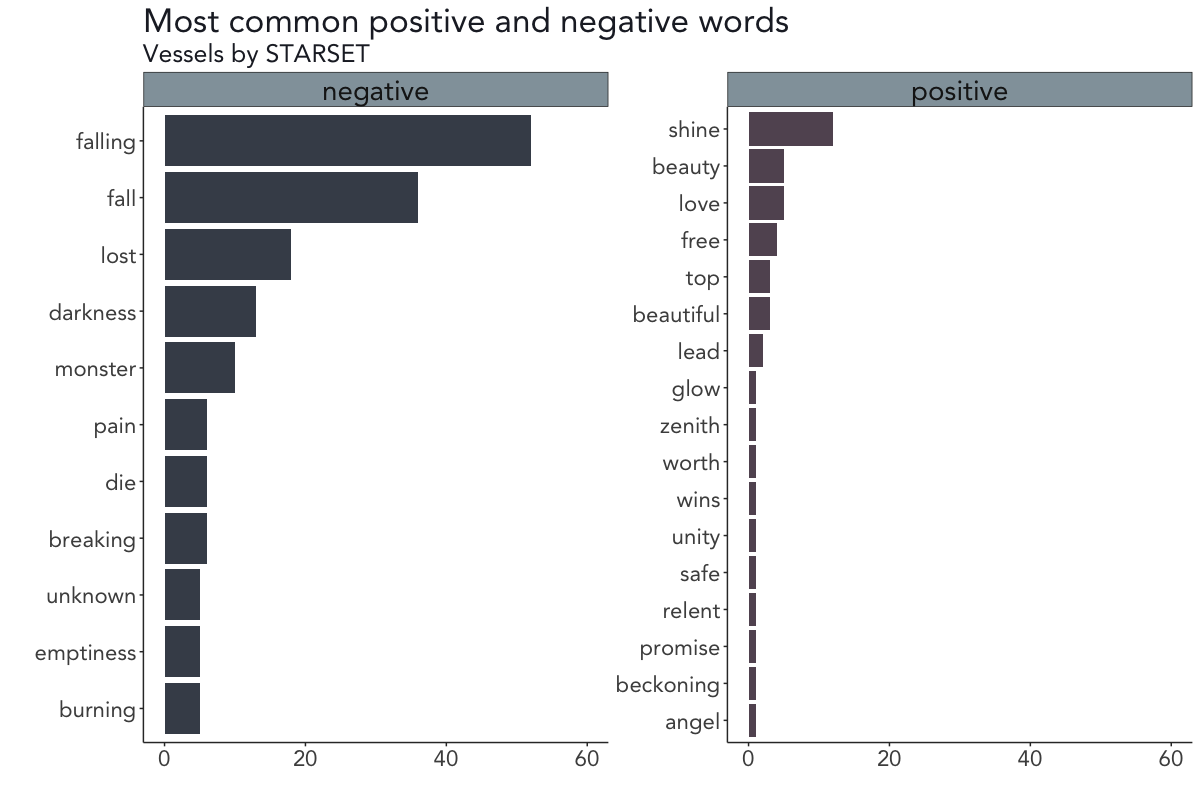
It seems as if not only the sentiments on both albums are strikingly similar but the most common words are as well.
On the debut album Transmissions, the words dark, fall, and lost (negatively scored) and free, love, and overtake (positively scored) occur most often, while the words falling, fall, and lost (negatively scored) and shine, beauty/love, and free are the most common words on the second album Vessels.
Calculating and visualizing n-grams
Up to this point, the analysis was based on words as individual units. When interested in co-occurring words or word sequences, you can go one step further and analyze the relationship between two (or more) words by tokenizing the song texts by pairs of adjacent words – so-called bigrams. See here for a more detailed explanation.
The next chunk of code extracts, counts, and visualizes these bigrams.
# Get bigrams with token = "ngrams" argument
starset_bigrams <- starset %>%
  group_by(album) %>%
  unnest_tokens(bigram, text, token = "ngrams", n = 2)

# Additional code to filter stop words from bigrams
starset_bigrams_sep <- starset_bigrams %>%
  separate(bigram, c("word1", "word2"), sep = " ")

starset_bigrams_filtered <- starset_bigrams_sep %>%
  filter(!word1 %in% stop_words$word) %>%
  filter(!word2 %in% stop_words$word)

starset_bigrams_united <- starset_bigrams_filtered %>%
  unite(bigram, word1, word2, sep = " ")

# Count bigrams based on unfiltered bigrams
starset_bigram_counts <- starset_bigrams %>%
  group_by(album) %>%
  count(bigram, sort = TRUE)

# Plot bigrams
starset_bigram_counts %>%
  group_by(album) %>%
  filter(n > 10) %>%
  ungroup() %>%
  mutate(bigram = reorder(bigram, n)) %>%
  ggplot(aes(bigram, n)) +
    geom_segment(aes(x = bigram,
                   xend = bigram,
                   y = 0,
                   yend = n), col = "grey50", alpha = 0.9) +
    geom_point(col = starset_cols[1:27], size = 4, alpha = 0.9) +
    facet_wrap(~album, scales = "free_y") +
    theme(text = element_text(size = 20, color = "#1f232e")) +
    xlab("") + ylab("") + ggtitle("Most common bigrams on STARSET albums", subtitle = " ") +
    ylim(0, 40) + coord_flip() + viz_theme

ggsave("plot5.png", width = 12, height = 8, units = "in", dpi = 100)
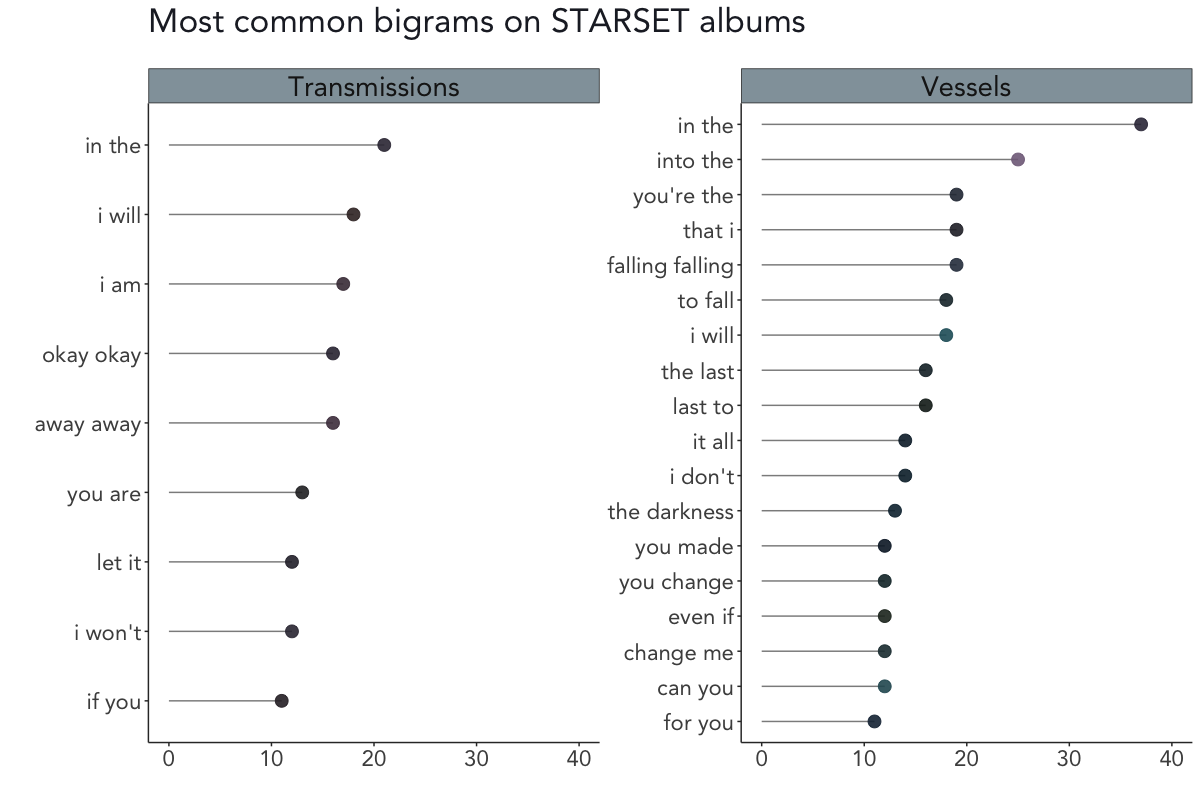
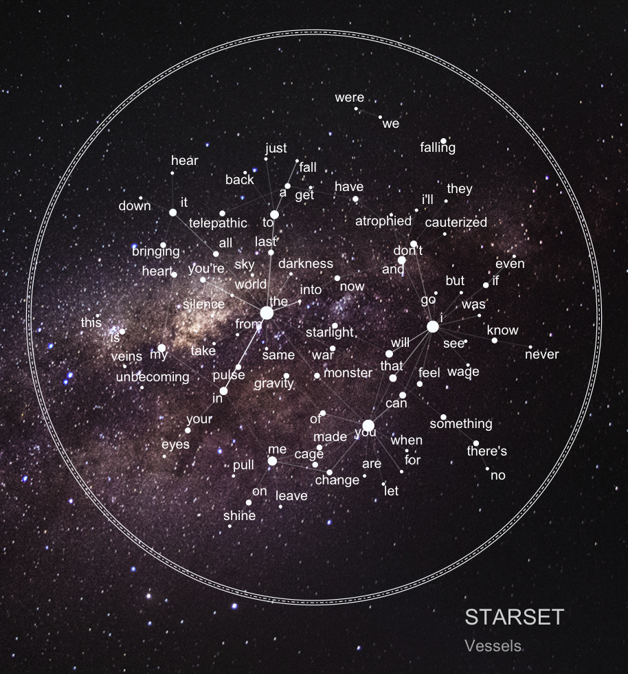
On Transmissions, the most common bigrams are in the, I will and I am (honorable mention to okay okay from My Demons, one of my favourite STARSET songs). On Vessels, the most common bigrams are in the, into the, and you’re the.
As is obvious from this list, I did not remove any stop words since there wouldn’t have been enough bigrams left for a sound analysis. However, I did include a snippet in the above code to filter stop words by splitting the bigrams into separate words, removing the stop words in each case, and merging them again. And just for the sake of completeness, the most common bigrams after removing the stop words were wanna break, fuel fanning, and break free on Transmissions and falling falling, telepathic heart and silence screams on Vessels.
Visualizing n-grams: Starplots
As mentioned in the introductory part of this post, I wanted to take up the idea of Nicholas Rougeux’s literary constellations which resulted in my so-called starplots (that are basically just simple space-themed bigram network graphs).
In order to create the starplots, I plotted bigram networks for each album on an image of the Milky Way and drew three circles with different linetypes around the nodes, based on the nodes’ respective coordinates.
When running the code below you should get these customized bigram networks, although you might have to play around a bit with the positioning aesthetics of the annotation layers as the nodes’ coordinates themselves aren’t fixed:
# Split bigrams by album and remove album column
starset_bigrams_tm <- starset_bigram_counts %>%
  filter(album == "Transmissions") %>%
  separate(bigram, c("word1", "word2"), sep = " ")
starset_bigrams_tm <- starset_bigrams_tm[, -1]

starset_bigrams_vs <- starset_bigram_counts %>%
  filter(album == "Vessels") %>%
  separate(bigram, c("word1", "word2"), sep = " ")
starset_bigrams_vs <- starset_bigrams_vs[, -1]

# Convert to igraph objects for plotting and filter by frequency
starset_bigram_tm_graph <- starset_bigram_tm %>%
  filter(n > 5) %>%
  graph_from_data_frame()

starset_bigram_vs_graph <- starset_bigram_vs %>%
  filter(n > 5) %>%
  graph_from_data_frame()

# Download background image
## Image credit: Marcio De Assis (https://commons.wikimedia.org/wiki/User:Marcio_De_Assis)
download.file("https://upload.wikimedia.org/wikipedia/commons/4/4d/Milky_Way_from_S%C3%A3o_Louren%C3%A7o.jpg", destfile = "milky_way.jpg", mode = "wb")

# Load picture and render
milky_way <- readJPEG("milky_way.jpg", native = TRUE)
milky_way <- rasterGrob(milky_way, interpolate = TRUE)

# Function to draw circles on plot
## Adapted from https://stackoverflow.com/questions/6862742/draw-a-circle-with-ggplot2.
## Thanks to Z. Lin over at Stack Overflow for helping me extending it!

gg_circle_from_position <- function(data, rsize = NA,
                                    color = "black", fill = NA,
                                    lty = NA, size = NA, ...){
  coord.x <- data[, "x"]
  coord.y <- data[, "y"]

  xc = mean(range(coord.x))
  yc = mean(range(coord.y))
  r = max(sqrt((coord.x - xc)^2 + (coord.y - yc)^2)) * rsize

  x <- xc + r*cos(seq(0, pi, length.out = 100))
  ymax <- yc + r*sin(seq(0, pi, length.out = 100))
  ymin <- yc + r*sin(seq(0, -pi, length.out = 100))
  annotate("ribbon", x = x, ymin = ymin, ymax = ymax,
           color = color, fill = fill, lty = lty, size = size, ...)
}

## Starplot: Transmissions
p <- ggraph(starset_bigram_tm_graph, layout = "fr") +
  annotation_custom(milky_way, xmin = -30, xmax = 30, ymin = -30, ymax = 30) +
  geom_edge_link(aes(edge_alpha = n*2), colour = "#fafdff") +
  geom_node_point(color = "#fafdff", aes(size = degree(starset_bigram_tm_graph)*8)) +
  geom_node_text(aes(label = name), color = "white", size = 5, check_overlap = TRUE, repel = TRUE,
                 nudge_x = 0.1, nudge_y = 0.1) +
  theme(panel.background = element_blank(),
        panel.grid.major = element_blank(),
        panel.grid.minor = element_blank(),
        axis.title = element_blank(),
        axis.text = element_blank(),
        axis.ticks.length = unit(0, "cm"),
        legend.position = "none")

p.positions <- layer_data(p, i = 2L)

p +
  gg_circle_from_position(data = p.positions, rsize = 1.23, color = "#fafdff", lty = 1, size = 0.4) +
  gg_circle_from_position(data = p.positions, rsize = 1.24, color = "#fafdff", lty = "3313", size = 0.4) +
  gg_circle_from_position(data = p.positions, rsize = 1.25, color = "#fafdff", lty = 1, size = 0.4) +
  annotate("text", x = 14, y = -4, hjust = 0, size = 8,
           label = paste("STARSET"), color = "white", alpha = 0.8) +
  annotate("text", x = 14, y = -5, hjust = 0, size = 6,
           label = paste("Transmissions"), color = "white", alpha = 0.6) +
  coord_equal()

ggsave("Starplot_Transmissions.png", width = 10, height = 10, units = "in", dpi = 100)

## Starplot: Vessels
p <- ggraph(starset_bigram_vs_graph, layout = "fr") +
  annotation_custom(milky_way, xmin = -30, xmax = 30, ymin = -30, ymax = 30) +
  geom_edge_link(aes(edge_alpha = n*2), colour = "#fafdff") +
  geom_node_point(color = "#fafdff", aes(size = degree(starset_bigram_vs_graph)*8)) +
  geom_node_text(aes(label = name), color = "white", size = 5, check_overlap = TRUE, repel = TRUE,
                 nudge_x = 0.1, nudge_y = 0.1) +
  theme(panel.background = element_blank(),
        panel.grid.major = element_blank(),
        panel.grid.minor = element_blank(),
        axis.title = element_blank(),
        axis.text = element_blank(),
        axis.ticks.length = unit(0, "cm"),
        legend.position = "none")

p.positions <- layer_data(p, i = 2L)

p +
  gg_circle_from_position(data = p.positions, rsize = 1.23, color = "#fafdff", lty = 1, size = 0.4) +
  gg_circle_from_position(data = p.positions, rsize = 1.24, color = "#fafdff", lty = "3313", size = 0.4) +
  gg_circle_from_position(data = p.positions, rsize = 1.25, color = "#fafdff", lty = 1, size = 0.4) +
  annotate("text", x = 10, y = -9, hjust = 0, size = 8,
           label = paste("STARSET"), color = "white", alpha = 0.8) +
  annotate("text", x = 10, y = -10, hjust = 0, size = 6,
           label = paste("Vessels"), color = "white", alpha = 0.6) +
  coord_equal()

ggsave("Starplot_Vessels.png", width = 10, height = 10, units = "in", dpi = 100)
![]()